DIGITAL TRANSFORMATION (DX) V/S FAKE TRANSFORMATION (FX)

 

KNOW THE DIFFERENCE

For those who don't like to read, here's the video:

In this new era that is ushering in the 4^th industrial revolution, almost every organization is seeking to adopt “Digital Transformation”. But today’s world is filled with fake transformation projects. A mere technology upgrade or change management do not account for authentic transformation. Organizations and leaders both in the public and private sector have been caught unaware with the “delusion of digital transformation”. Many of the projects that CEOs and other leaders undertake are akin to moving from traditional systems to paperless office or shifting from legacy to cloud infrastructure. They are victims of this grand delusion and will eventually lead their organizations to an early grave.

Digital Transformation (DT or DX) is the adoption of digital technology to transform services or businesses, through replacing non-digital or manual processes with digital processes or replacing older digital technology with newer digital technology. Digital solutions may enable - in addition to efficiency via automation - new types of innovation and creativity, rather than simply enhancing and supporting traditional methods. (Source: https://en.wikipedia.org/wiki/Digital_transformation)

Digital Transformation is application of digital capabilities to processes, products, and assets to improve efficiency, enhance customer value, manage risk, and uncover new monetization opportunities. (Source: https://www.cio.com/article/3199030/what-is-digital-transformation.html)

Researchers have analyzed some digital transformation strategy examples and trends of recent years.

Eventually, some of the key predictions were:

·         By 2023, investments in digital transformation will grow from 36% in 2019 to over 50% of all information and communication technology investments.

·         Investments in direct digital transformations are rapidly growing at an annual rate of 17.5%. They’re expected to approach $7.4 trillion over 2020-2023.

·         By 2024, artificial intelligence-powered companies will respond to their customers and partners 50% faster than their peers.

(Source: IDC FutureScape: Worldwide Digital Transformation 2020 Predictions, October 2019)

The idea is to create whole new products, services or business models, not just improve old ones. Companies that go through digital transformation are said to be more agile, customer centric and data driven. DX can have different blueprints depending upon the company and industry. But, in all cases it needs to follow these basic steps:

In terms of the People-Process-Technology framework, a definite “cultural shift” is a prerogative to achieve DX in its truest sense. Businesses must learn to push boundaries, experiment, and accept the associated failures. This potentially involves abandoning well-established processes for new ones – ones that are often still being defined.

For real DX, one needs to separate from the herd involved in FX.

Look at the chart given below:

It doesn’t matter if you find yourself in quadrant one, but never stray from the course that turns out to be an FX instead of genuine DX. A few good examples of DX are given below for you to understand and get inspired:

Anheuser-Busch (AB) InBev has looked at how digital transformation can be applied all through the business while retaining focus on serving its consumers. They have achieved it via the following –

·         Developed a mobile application called B2B with an inbuilt algorithm that makes specific replenishment suggestions, creating opportunities for sales staff to talk about new brands and products with store owners.

·         Created a tech innovation lab, Beer Garage, to explore ways that artificial intelligence (AI), machine learning (ML) and the internet of things (IoT), among other technologies can be used to improve experiences for consumers and retailers alike.

DHL is well known for its excellent stock management and supply chain but that did not stop them from improving. Their stock management and supply chain systems are easy to use and automated, but they want to take things to the next level. For this they decided to team up with Ricoh and Ubimax and –

·         Developed application for smart glasses. By pairing smart glasses with these applications, it can be used for reading bar codes, streamline pickup and drop off and reduce the chances of errors. Their stock price doubled from 20 euros in 2016 to 40 euros in 2018.

Honeywell has helped many companies improve their digital presence and capabilities. In 2016 the company began transforming itself digitally by introducing new technologies like data-centric, internet-connected, offerings and devices. They have leveraged digital solutions like this –

·         Using new digitized internal solutions and customer data, the company now offers its customers more technology solutions and has reinvented its industrial process control. As a result, in the past four years, Honeywell’s stock per share price has gone from $95 to $174.

As a leader what you must be doing is listed below:

·         Develop competency – Invest in talent and upgrading skills of employees in the organization. Digital and analytics skills are very critical for DX and go a long way in bringing about real transformation.

·         Plan and prioritize – Assess the current scenario and develop a roadmap. An efficient plan makes a solid foundation for any achievement. Pick relevant themes and prepare a business case.

·         Commitment – Absolute commitment along with appropriate investment is crucial to bring about DX. Always look at the tangible as well as intangible benefits of the project.

A snapshot for a typical CDO is provided below:

Hence, the message is to steer clear of all types of fake transformation projects and drive real digital transformation projects that truly alter the arena. I can conclude this article with an allegorical anecdote:

Resume statement (DX)	Reality (FX)
Surpassed targets by 60% through implementing energy saving initiatives and loss prevention strategies via leading digital transformation projects across the organization, thereby contributing to the bottom line of the company.

Note: This blog including all articles are copyrighted by the author. Wherever, external content is used, the relevant sources are posted in separate links or the images itself. 

PREDICTIVE ANALYTICS FOR THE ENERGY SECTOR

 

Machine Learning Business Use Case

One of the major areas where AIML can truly change the landscape is the energy sector. Let us first understand the “Analytics Maturity Model” before attempting to consider the implications:

Almost all the OEMs and principals of the energy sector have in-built objective analytics (e.g. enterprise pipeline management solution) along with ICS / DCS since ages that address the essential process requirements like vibration monitoring, condition monitoring, cathodic protection etal. pertaining to asset integrity. Then, we also have the major players that have developed real-time monitoring solutions in pace with the 4^th industrial revolution viz. advanced telemetry, imaging systems, distributed monitoring systems (vibration, acoustics, temperature), etc. However, when it comes to predictive analytics there is a huge gap since it is mostly done in hind-sight and is not real-time. There are very few players in the market who have indeed rolled-out real-time predictive analytics either as a SaaS model or a standalone offering. The GTM feasibility of many other similar products is underway as the global MLaaS market is forecasted to reach USD 117.19 billion by 2027 (source: https://www.fortunebusinessinsights.com/machine-learning-market-102226).   

Use-case Scenario

For the energy sector, there can be several use-case scenarios as listed below:

•  Process Optimization
•  Reducing MTBF / MTTR
•  Loss Prevention (process losses, leakages, etc.)

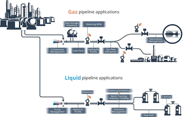
Here, I will attempt to present a use case scenario for “real-time predictive analytics” for a typical natural gas pipeline. A typical high-level production process flow is given below:

 

In this example, let us presume that we have a simple process flow for pipeline data management as shown below:

Data Scientists / Analysts must be aware of the entire data science life-cycle before attempting to initiate the solution as shown below:

Once the logged data is collected, the machine learning process is initiated as per the process flow shown below:

It is to be noted that supervised learning models are preferred since OEM design parameters need to be considered for baseline / target values. However, semi-supervised algorithms may be used while using a classification approach to get better results.

Building the model

Remember that the processed data will be humongous with hundreds of columns to accommodate all the relevant parameters collected via numerous sensors required to maintain pipeline integrity. Here, I will be focusing only on semi-supervised graph-based algorithms that can be validated and finally selected for deployment. For ease of business, I’m only considering distributed temperature monitoring dataset in this case.

Label Spreading

It is based on the normalized graph Laplacian:

This matrix has each a diagonal element l_ii equal to 1, if the degree deg(l_ii) > 0 (0 otherwise) and all the other elements equal to:

The behavior of this matrix is analogous to a discrete Laplacian operator, whose real-value version is the fundamental element of all diffusion equations. To better understand this concept, let's consider the generic heat equation:

This equation describes the behavior of the temperature of a pipeline section when a point is suddenly heated. From basic physics concepts, we know that heat will spread until the temperature reaches an equilibrium point and the speed of variation is proportional to the Laplacian of the distribution. If we consider a bidimensional grid at the equilibrium (the derivative with respect to when time becomes null) and we discretize the Laplacian operator (∇² = ∇ * ∇) considering the incremental ratios, we obtain:

Therefore, at the equilibrium, each point has a value that is the mean of the direct neighbors. It's possible to prove the finite-difference equation has a single fixed point that can be found iteratively, starting from every initial condition. In addition to this idea, label spreading adopts a clamping factor α for the labeled samples. If α=0, the algorithm will always reset the labels to the original values (like for label propagation), while with a value in the interval (0, 1], the percentage of clamped labels decreases progressively until α=1, when all the labels are overwritten.

The complete steps of the label spreading algorithm are:

•         Select an affinity matrix type (KNN or RBF) and compute W
•         Compute the degree matrix D
•         Compute the normalized graph Laplacian L
•         Define Y⁽⁰⁾ = Y
•         Define α in the interval [0, 1]
•         Iterate until convergence of the following step –

It's possible to show that this algorithm is equivalent to the minimization of a quadratic cost function with the following structure:

The first term imposes consistency between original labels and estimated ones (for the labeled samples). The second term acts as a normalization factor, forcing the unlabeled terms to become zero, while the third term, which is probably the least intuitive, is needed to guarantee geometrical coherence in terms of smoothness.

Python code for Label Spreading

We can test this algorithm using the Scikit-Learn implementation. Let's start by creating a very dense dataset:

from sklearn.datasets import make_classification

nb_samples = 5000 nb_unlabeled = 1000

X, Y = make_classification(n_samples=nb_samples, n_features=2,

n_informative=2, n_redundant=0, random_state=100)

Y[nb_samples - nb_unlabeled:nb_samples] = -1

We can train a LabelSpreading instance with a clamping factor alpha=0.2. We want to preserve 80% of the original labels but, at the same time, we need a smooth solution:

from sklearn.semi_supervised import LabelSpreading

ls = LabelSpreading(kernel='rbf', gamma=10.0, alpha=0.2)

ls.fit(X, Y)

Y_final = ls.predict(X)

The result is shown, as usual, together with the original dataset:

As it's possible to see in the first figure (left), in the central part of the cluster (x [-1, 0]), there's an area of circle dots. Using a hard-clamping, this aisle would remain unchanged, violating both the smoothness and clustering assumptions. Setting α > 0, it's possible to avoid this problem. Of course, the choice of α is strictly correlated with each single problem. If we know that the original labels are absolutely correct, allowing the algorithm to change them can be counterproductive. In this case, for example, it would be better to preprocess the dataset, filtering out all those samples that violate the semi-supervised assumptions. If, instead, we are not sure that all samples are drawn from the same pdata, and it's possible to be in the presence of spurious elements, using a higher α value can smooth the dataset without any other operation.

Similarly, one can also use “Label Propagation based on Markov Random Walks” to find the probability distribution of target labels for unlabeled samples given a mixed dataset by simulation of stochastic process.

It is to be noted that the above two algorithms can be applied against design parameters adjusted against the best achieved values based on historical data. In any other scenario, the predictions may go totally wrong since the iterations are based on absolute correctness of the labels (e.g. derived from control limits or stability tests).

Once the model has been validated with good level of accuracy and deployed for production, the ICS (Industrial Control System) interface (API integration) for real-time predictive analytics can be set-up that will trigger alarms at the set control points and provide deeper insights for loss prevention. As the ML system matures over time, one may even be able to move to the next level i.e. “Prescriptive Analytics”.

Conclusion

Given below is a estimated annual cost for the minimum length (100 km) and minimum diameter (12 inch) of a large company:

Component	Segment A (small)	Segment B (large)	Total
Periodic Inspection	$ 121550	$ 297000	$ 418550
Scheduled Pigging	$ 40000	$ 80000	$ 120000
Leak Surveys (@95% of total)	$ 13000	$ 22000	$ 35000
Repair Backlog (@annual cost of rule)	$ 103000	$ 197000	$ 300000
Total	$ 277550	$ 596000	$ 873550

Source: Greene’s Energy Group, LLC (2013), updated to 2015 dollars using the Bureau of Labor Statistics US All City Average Consumer Price Index (2013=233.5; 2015=237.8).

Note: The above table is a simplified one and does not include several factors like terrain, regulated / unregulated, mobilization costs, compliance costs, etc.

Cost-benefit Analysis

It is to be noted that even a 1% of loss prevention against an average production of 6 MMSCFD (169512.82 m3/d or 1066203.53 bbl/d) goes a long way in cost optimization for an oil & gas producer.

For this particular example, a savings of US$ 5400 / km can be easily achieved for a combined loss prevention strategy (gathering / process loss & maintenance / inspection cost).

Note: The above is a highly conservative estimate and actual savings may be 4x higher in actual practice. 

Reference Standards: ISO 55001:2014 Asset Management, ISO 31000:2018 Risk Management, ISO 14224:2006 Petroleum, petrochemical and natural gas reliability & maintenance, ISO/IEC CD 22989 AI Terms & Concepts, ISO/IEC AWI TR 5469 AI Functional Safety

Pitfalls to avoid for effective model building

Watch this video about this article:

It is of utmost importance that the most optimized model is deployed for production and this is usually done via model performance characteristics like accuracy, precision, recall, f1 score, etc. To achieve this, we may employ various methods like feature engineering, hyper-parameter tuning, SVMs, etc.

However, before optimizing any model, we need to choose the right one in the first place. There are several factors that come into play before we decide upon the suitability of any model like:

a.     Has the data been cleaned adequately?

b.     What methods have been used for data preparation?

c.      What feature engineering techniques are we going to apply?

d.     How do we interpret and handle the observations like skewness, outliers, etc.?

Here, we will focus on the last factor mentioned above where most of us are prone to commit mistakes.

It is a standard practice to normalize the distribution by reducing the outliers, dropping certain parameters, etc. before feature selection. But, sometimes one might need to take a step back and observe –

a.     How is our normalization affecting the entire dataset and

b.     Is it gearing us towards the correct solution within the given context?

Let us examine this premise with a practical example as shown below.

Problem statement: Predicting concrete cement compressive strength using artificial neural networks

As usual, the data has been cleaned and prepared for detailed analysis before going for model selection and building. Please note that, we will not be addressing the initial stages in this article. Let us have a look at some of the key steps and observations as described below.

1.     Dropping outliers for normalization

An initial exploratory data analysis and visualization depicts the overall distribution of the target column “strength” -

As seen above, the data distribution is quite sparse with multiple skewness, both positive and negative. Further analysis reveals the following:

The following are the observations:

a.   Cement, slag, ash, courseagg and fineagg display huge differences indicating possibility of outliers

b.     Slag, ash and coarseagg have their median values closer to either 1st quartile or minimum values while both slag and fineagg have maximum values as outliers.

c.      Target column "strength" has many maximum values as outliers.

Replacing outliers for Concrete Cement Compressive Strength with any other value will beat the purpose of the data analysis i.e. develop a best fit model that gives an appropriate mixture with “maximum compressive strength”. Hence, it is good to replace outliers with mean values only for other variables as per the analysis and leave the target column as it is.

2.     Dropping variables to reduce skewness

Before applying feature engineering techniques, we need to look at correlation of the variables as shown below:

Observations based on our analysis:

a.     There is no high correlation between any of the variables

b.     Compressive strength increases with amount of cement

c.      Compressive strength increases with age

d.     As fly-ash increases the compressive strength decreases

e.     Strength increases with addition of Superplasticizer

Observations based on domain knowledge:

a.     Cement with low age requires more water for higher strength i.e. older the cement, more the water it requires

b.     Strength increases when less water is used in preparing it i.e. more of water leads to reduced strength

c.      Less of coarse aggregate along with less of slag increases strength

We can drop the variable slag only while the rest need to be retained.  

If we were to drop certain variables solely based on observed correlation in the given dataset, we would end up with a model having pretty high accuracy but at the same time it would be considered at best a “paper model” i.e. not practicable in the real world. Hence, certain amount of domain knowledge either directly or through consultation with a subject-matter expert goes a long way in avoiding major pitfalls while model building. 

The above example pretty much sums up, what we can call as “bias” (pun intended) that most of us can be prone to whether we are having a technical edge or a domain edge. Hence, it is a good practice to rethink the methods applied vis-à-vis the big picture.

Source:  The data for this project is available in file https://archive.ics.uci.edu/ml/machine-learning-databases/concrete/compressive/

Reference:  I-Cheng Yeh, "Modeling of strength of high performance concrete using artificial neural networks," Cement and Concrete Research, Vol. 28, No. 12, pp. 1797-1808 (1998).

 

AI Ethics

#AIML

The industrial revolution 4.0 is ushering in a new era of change across all spheres of our lives. With the emergence of artificial intelligence and machine learning (AIML) mankind is taking huge leaps into the unknown future.

AIML is touching everyone's lives directly or indirectly in myriad ways. Whether, it is an advertisement that pops-up on your screen or the traffic lights that you see on the streets, it's constantly influencing you all the time. At a broader level AIML might even influence what you would buy at the supermarket or to which candidate your vote goes to. In today's world with pervasive technology, it's hard to determine who's in control?

That brings us to the grand question of AI ethics. Any technological advancement must serve its primary purpose viz. filling the gap either via solving a problem or fulfilling a need. However, this purpose cannot be achieved at the expense of its beneficiary i.e. consumer. AIML helps organizations to achieve the goal via data manipulation. So far, so good. The primary input i.e. data needs to be reliable, comprehensible, and realistic to be of any use. But, it must also be obtained via fair means i.e. it must not infringe upon any legal or moral codes.

How often do organizations ensure this?

To be continued...

Watch the video here: